Output: Multinomial Logit model

Posterior means, posterior standard deviations and 95% credible intervals (Inference->Samples->stats)

*Pr(Correct classification | data) =0.813, Pr(Correct classification for category 1| data) =0.754,

Pr(Correct classification for category 2| data) =0.804, Pr(Correct classification for category 3| data) =0.845.

Sample path (history)

Posterior probability densities (Inference->Samples->density)

(Further, right click on the figure->Margins-> Special…->Smooth -> change from 0.2 to 0.1-> apply all)

Sample autocorrelation function (Inference->Samples->auto corr)

Running quantile plot (Inference->Samples->quantiles)

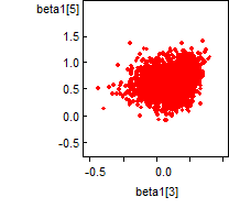
Scatter plots (Inference->Correlations…) Enter “beta1” (or “beta3”) in node box and click on scatter.

Scatter plots (Inference->Correlations…) Enter “beta1” (or “beta3”) in node box and click on matrix.

Prediction : Pr(category 1 | log(cash flow), other independent variables (at their means), data)

(Inference-> Compare-> node:pp[,1], axis:p.lcf, and click on modelfit)

(Further, right-click on the figure, Titles -> x-axis: log(cash flow), title: Pr(category 1|data))

95% intervals (blue) and median (red)

Prediction : Pr(category 2| log(cash flow), other independent variables (at their means), data)

(Inference-> Compare-> node:pp[,2], axis:p.lcf, and click on modelfit)

(Further, right-click on the figure, Titles -> x-axis: log(cash flow), title: Pr(category 2|data))

95% intervals (blue) and median (red)

Prediction : Pr(category 3| log(cash flow), other independent variables (at their means), data)

(Inference-> Compare-> node:pp[,2], axis:p.lcf, and click on modelfit)

(Further, right-click on the figure, Titles -> x-axis: log(cash flow), title: Pr(category 3|data))

95% intervals (blue) and median (red)